Element Reference
Passives
ACME.resistor — Functionresistor(r)Creates a resistor obeying Ohm’s law. The resistance r has to be given in Ohm.
Pins: 1, 2
ACME.capacitor — Functioncapacitor(c)Creates a capacitor. The capacitance c has to be given in Farad.
Pins: 1, 2
ACME.inductor — Methodinductor(l)Creates an inductor. The inductance l has to be given in Henri.
Pins: 1, 2
ACME.inductor — Methodinductor(Val{:JA}; D, A, n, a, α, c, k, Ms)Creates a non-linear inductor based on the Jiles-Atherton model of magnetization assuming a toroidal core thin compared to its diameter. The parameters are set using named arguments:
| parameter | description |
|---|---|
D | Torus diameter (in meters) |
A | Torus cross-sectional area (in square-meters) |
n | Winding's number of turns |
a | Shape parameter of the anhysteretic magnetization curve (in Ampere-per-meter) |
α | Inter-domain coupling |
c | Ratio of the initial normal to the initial anhysteretic differential susceptibility |
k | amount of hysteresis (in Ampere-per-meter) |
Ms | saturation magnetization (in Ampere-per-meter) |
A detailed discussion of the parameters can be found in D. C. Jiles and D. L. Atherton, “Theory of ferromagnetic hysteresis,” J. Magn. Magn. Mater., vol. 61, no. 1–2, pp. 48–60, Sep. 1986 and J. H. B. Deane, “Modeling the dynamics of nonlinear inductor circuits,” IEEE Trans. Magn., vol. 30, no. 5, pp. 2795–2801, 1994, where the definition of c is taken from the latter. The ACME implementation is discussed in M. Holters, U. Zölzer, "Circuit Simulation with Inductors and Transformers Based on the Jiles-Atherton Model of Magnetization".
Pins: 1, 2
ACME.transformer — Methodtransformer(l1, l2; coupling_coefficient=1, mutual_coupling=coupling_coefficient*sqrt(l1*l2))Creates a transformer with two windings having inductances. The primary self-inductance l1 and the secondary self-inductance l2 have to be given in Henri. The coupling can either be specified using coupling_coefficient (0 is not coupled, 1 is closely coupled) or by mutual_coupling, the mutual inductance in Henri, where the latter takes precedence if both are given.
Pins: primary1 and primary2 for primary winding, secondary1 and secondary2 for secondary winding
ACME.transformer — Methodtransformer(Val{:JA}; D, A, ns, a, α, c, k, Ms)Creates a non-linear transformer based on the Jiles-Atherton model of magnetization assuming a toroidal core thin compared to its diameter. The parameters are set using named arguments:
| parameter | description |
|---|---|
D | Torus diameter (in meters) |
A | Torus cross-sectional area (in square-meters) |
ns | Windings' number of turns as a vector with one entry per winding |
a | Shape parameter of the anhysteretic magnetization curve (in Ampere-per-meter) |
α | Inter-domain coupling |
c | Ratio of the initial normal to the initial anhysteretic differential susceptibility |
k | amount of hysteresis (in Ampere-per-meter) |
Ms | saturation magnetization (in Ampere-per-meter) |
A detailed discussion of the parameters can be found in D. C. Jiles and D. L. Atherton, “Theory of ferromagnetic hysteresis,” J. Magn. Magn. Mater., vol. 61, no. 1–2, pp. 48–60, Sep. 1986 and J. H. B. Deane, “Modeling the dynamics of nonlinear inductor circuits,” IEEE Trans. Magn., vol. 30, no. 5, pp. 2795–2801, 1994, where the definition of c is taken from the latter. The ACME implementation is discussed in M. Holters, U. Zölzer, "Circuit Simulation with Inductors and Transformers Based on the Jiles-Atherton Model of Magnetization".
Pins: 1 and 2 for primary winding, 3 and 4 for secondary winding, and so on
Independent Sources
ACME.voltagesource — Functionvoltagesource(; rs=0)
voltagesource(v; rs=0)Creates a voltage source. The source voltage v has to be given in Volt. If omitted, the source voltage will be an input of the circuit. Optionally, an internal series resistance rs (in Ohm) can be given which defaults to zero.
Pins: + and - with v being measured from + to -
ACME.currentsource — Functioncurrentsource(; gp=0)
currentsource(i; gp=0)Creates a current source. The source current i has to be given in Ampere. If omitted, the source current will be an input of the circuit. Optionally, an internal parallel conductance gp (in Ohm⁻¹) can be given which defaults to zero.
Pins: + and - where i measures the current leaving source at the + pin
Probes
ACME.voltageprobe — Functionvoltageprobe()Creates a voltage probe, providing the measured voltage as a circuit output. Optionally, an internal parallel conductance gp (in Ohm⁻¹) can be given which defaults to zero.
Pins: + and - with the output voltage being measured from + to -
ACME.currentprobe — Functioncurrentprobe()Creates a current probe, providing the measured current as a circuit output. Optionally, an internal series resistance rs (in Ohm) can be given which defaults to zero.
Pins: + and - with the output current being the current entering the probe at +
Semiconductors
ACME.diode — Functiondiode(;is=1e-12, η = 1)Creates a diode obeying Shockley's law $i=I_S\cdot(e^{v/(\eta v_T)}-1)$ where $v_T$ is fixed at 25 mV. The reverse saturation current is has to be given in Ampere, the emission coefficient η is unitless.
Pins: + (anode) and - (cathode)
ACME.bjt — Functionbjt(typ; is=1e-12, η=1, isc=is, ise=is, ηc=η, ηe=η, βf=1000, βr=10,
ile=0, ilc=0, ηcl=ηc, ηel=ηe, vaf=Inf, var=Inf, ikf=Inf, ikr=Inf)Creates a bipolar junction transistor obeying the Gummel-Poon model
\[i_f = \frac{\beta_f}{1+\beta_f} I_{S,E} \cdot (e^{v_E/(\eta_E v_T)}-1)\]
\[i_r = \frac{\beta_r}{1+\beta_r} I_{S,C} \cdot (e^{v_C/(\eta_C v_T)}-1)\]
\[i_{cc} = \frac{2(1-\frac{V_E}{V_{ar}}-\frac{V_C}{V_{af}})} {1+\sqrt{1+4(\frac{i_f}{I_{KF}}+\frac{i_r}{I_{KR}})}} (i_f - i_r)\]
\[i_{BE} = \frac{1}{\beta_f} i_f + I_{L,E} \cdot (e^{v_E/(\eta_{EL} v_T)}-1)\]
\[i_{BC} = \frac{1}{\beta_r} i_r + I_{L,C} \cdot (e^{v_C/(\eta_{CL} v_T)}-1)\]
\[i_E = i_{cc} + i_{BE} \qquad i_C=-i_{cc} + i_{BC}\]
where $v_T$ is fixed at 25 mV. For
\[I_{L,E}=I_{L,C}=0,\quad V_{ar}=V_{af}=I_{KF}=I_{KR}=∞,\]
this reduces to the Ebers-Moll equation
\[i_E = I_{S,E} \cdot (e^{v_E/(\eta_E v_T)}-1) - \frac{\beta_r}{1+\beta_r} I_{S,C} \cdot (e^{v_C/(\eta_C v_T)}-1)\]
\[i_C = -\frac{\beta_f}{1+\beta_f} I_{S,E} \cdot (e^{v_E/(\eta_E v_T)}-1) + I_{S,C} \cdot (e^{v_C/(\eta_C v_T)}-1).\]
Additionally, terminal series resistances are supported.
The parameters are set using named arguments:
| parameter | description |
|---|---|
typ | Either :npn or :pnp, depending on desired transistor type |
is | Reverse saturation current in Ampere |
η | Emission coefficient |
isc | Collector reverse saturation current in Ampere (overriding is) |
ise | Emitter reverse saturation current in Ampere (overriding is) |
ηc | Collector emission coefficient (overriding η) |
ηe | Emitter emission coefficient (overriding η) |
βf | Forward current gain |
βr | Reverse current gain |
ilc | Base-collector junction leakage current in Ampere |
ile | Base-emitter junction leakage current in Ampere |
ηcl | Base-collector junction leakage emission coefficient (overriding η) |
ηel | Base-emitter junction leakage emission coefficient (overriding η) |
vaf | Forward Early voltage in Volt |
var | Reverse Early voltage in Volt |
ikf | Forward knee current (gain roll-off) in Ampere |
ikr | Reverse knee current (gain roll-off) in Ampere |
re | Emitter terminal resistance |
rc | Collector terminal resistance |
rb | Base terminal resistance |
Pins: base, emitter, collector
ACME.mosfet — Functionmosfet(typ; vt=0.7, α=2e-5, λ=0)Creates a MOSFET transistor with the simple model
\[i_D=\begin{cases} 0 & \text{if } v_{GS} \le v_T \\ \alpha \cdot (v_{GS} - v_T - \tfrac{1}{2}v_{DS})\cdot v_{DS} \cdot (1 + \lambda v_{DS}) & \text{if } v_{DS} \le v_{GS} - v_T \cap v_{GS} > v_T \\ \frac{\alpha}{2} \cdot (v_{GS} - v_T)^2 \cdot (1 + \lambda v_{DS}) & \text{otherwise.} \end{cases}\]
The typ parameter chooses between NMOS (:n) and PMOS (:p). The threshold voltage vt is given in Volt, α (in A/V²) is a constant depending on the physics and dimensions of the device, and λ (in V⁻¹) controls the channel length modulation.
Optionally, it is possible to specify tuples of coefficients for vt and α. These will be used as polynomials in $v_{GS}$ to determine $v_T$ and $\alpha$, respectively. E.g. with vt=(0.7, 0.1, 0.02), the $v_{GS}$-dpendent threshold voltage $v_T = 0.7 + 0.1\cdot v_{GS} + 0.02\cdot v_{GS}^2$ will be used.
Pins: gate, source, drain
Integrated Circuits
ACME.opamp — Methodopamp(;maxgain=Inf, gain_bw_prod=Inf)Creates a linear operational amplifier as a voltage-controlled voltage source. The input current is zero while the input voltage is mapped to the output voltage according to the transfer function
\[H(f) = \frac{A_\text{max}}{\sqrt{A_\text{max}^2-1} i \frac{f}{f_\text{UG}} + 1}\]
where $f$ is the signal frequency, $A_\text{max}$ (maxgain) is the maximum open loop gain and $f_\text{UG}$ (gain_bw_prod) is the gain/bandwidth product (unity gain bandwidth). For gain_bw_prod=Inf (the default), this corresponds to a frequency-independent gain of maxgain. For maxgain=Inf (the default), the amplifier behaves as a perfect integrator.
For both maxgain=Inf and gain_bw_prod=Inf, i.e. just opamp(), an ideal operational amplifier is obtained that enforces the voltage between the input pins to be zero while sourcing arbitrary current on the output pins without restricting their voltage.
Note that the opamp has two output pins, where the negative one will typically be connected to a ground node and has to provide the current sourced on the positive one.
Pins: in+ and in- for input, out+ and out- for output
ACME.opamp — Methodopamp(Val{:macak}, gain, vomin, vomax)Creates a clipping operational amplifier where input and output voltage are related by
\[v_\text{out} = \frac{1}{2}\cdot(v_\text{max}+v_\text{min}) +\frac{1}{2}\cdot(v_\text{max}-v_\text{min})\cdot \tanh\left(\frac{g}{\frac{1}{2}\cdot(v_\text{max}-v_\text{min})}\cdot v_\text{in}\right).\]
The input current is zero, the output current is arbitrary.
Note that the opamp has two output pins, one of which will typically be connected to a ground node and has to provide the current sourced on the other output pin.
Pins: in+ and in- for input, out+ and out- for output
Adding custom elements
One advantage of ACME is that it is relatively easy to define one's own circuit elements. However, the required formalism is a bit non-obvious. So this section is meant to be an introduction into steps required to implement a custom circuit element. As a running example, we shall consider an operational transconductance amplifier (OTA). As the name suggests, it is similar to an operation amplifier in that it has two input pins, acting as a differential input, and a single output pin. For the OTA, the output current is (approximately) proportional to the differential input voltage. The factor of proportionality (transconductance) can be controlled by the current drawn at a further pin. Additionally, the OTA has power supply pins, of course.
We shall start with a simple linear model with fixed transconductance. We idealize the input current to be zero adn the output voltage as arbitrary, i.e. the OTA acts as an ideal, voltage-controlled current source. The first step is to define the ports (pairs of pins) of the element, such that the behavior of the element can be defined in terms of the voltages across and currents through these ports. For the OTA, the first port can obviously be chosen as the input pins. For the second port, the output pin has to be paired with a pin that provides the current to be sourced at the output to maintain a net current sum of zero. As for the opamp models, we therefore introduce a negative output pin. Each port is associated with a voltage and a current as depicted in the following diagram:
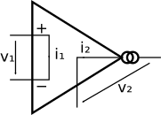
The OTA is thus described with $i_2=-g\cdot v_1$ (where $g$ is the transconductance) and $i_1=0$. The negative sign in the first equation is required because we want a positive input voltage to yield a positive output current pointing out of the OTA, i.e. opposite to $i_2$.
ACME uses a matrix notation that in full generality looks like
\[\bm{M}_\text{v}\bm{v} + \bm{M}_\text{i}\bm{i} + \bm{M}_\text{x}\bm{x} + \bm{M}_{\dot{\text{x}}}\dot{\bm{x}} + \bm{M}_\text{q}\bm{q} = \bm{M}_\text{u}\bm{u} + \bm{u}_0.\]
The matrices $\bm{M}_{\cdot}$ describe the element and will have to be determined in the following. The port voltages and currents are collected in vectors $\bm{v}$ and $\bm{i}$, respectively. The vector $\bm{x}$ holds the internal states of the element and $\dot{\bm{x}}$ their derivatives. We model a stateless OTA, so these parts can be ignored by choosing $\bm{M}_\text{x}$ and $\bm{M}_{\dot{\text{x}}}$ as zero-column matrices. The vector $\bm{q}$ becomes relevant for nonlinear elements, but can likewise be ignored for the moment choosing $\bm{M}_\text{q}$ as a zero-column matrix. The vector $\bm{u}$ contains externally controlled inputs, which we don't have for the OTA, so $\bm{M}_\text{u}$ is also chosen to have zero columns. Finally, $\bm{u}_0$ is again used for describing the element. For the linear OTA, we can write the two equations as
\[\underbrace{\begin{pmatrix} g & 0 \\ 0 & 0 \end{pmatrix}}_{\bm{M}_\text{v}} \cdot\underbrace{\begin{pmatrix} v_1 \\ v_2 \end{pmatrix}}_{\bm{v}} + \underbrace{\begin{pmatrix} 0 & 1 \\ 1 & 0 \end{pmatrix}}_{\bm{M}_\text{i}} \cdot\underbrace{\begin{pmatrix} i_1 \\ i_2 \end{pmatrix}}_{\bm{i}} = \underbrace{\begin{pmatrix} 0 \\ 0 \end{pmatrix}}_{\bm{u}_0}\]
where the first row translates to $i_2=-g\cdot v_1$ and the second row to $i_1=0$. Thus, we obtain
\[\bm{M}_\text{v}=\begin{pmatrix} g & 0 \\ 0 & 0 \end{pmatrix} \quad \bm{M}_\text{i} = \begin{pmatrix} 0 & 1 \\ 1 & 0 \end{pmatrix} \quad \bm{u}_0 = \begin{pmatrix} 0 \\ 0 \end{pmatrix}.\]
Translation to ACME is straight-forward, as the Element constructor takes self-explanatorily named keyword arguments:
g=10e-3
ACME.Element(mv=[g 0; 0 0], mi=[0 1; 1 0],  ports=["in+" => "in-", "out+" => "out-"])
Omitted matrices are taken to be empty/all-zero matrices of suitable size. The ports are specified as pairs of pins. The names can be chosen arbitrarily. If the same pin name is used in multiple ports, these ports share a pin. For example, the bjt has a base-collector and a base-emitter port, sharing base as a common pin.
It is usually convenient to wrap the element creation in a suitable function like it is done for the elements defined as part of ACME:
ota(g) = ACME.Element(mv=[g 0; 0 0], mi=[0 1; 1 0], ports=["in+" => "in-", "out+" => "out-"])A simple test circuit for this OTA could then be run with
circ = @circuit begin
    Jin = voltagesource()
    U = ota(10e-3), ["in+"] ⟷ Jin[+], ["in-"] ⟷ Jin[-]
    Jout = currentprobe(), [+] ⟷ U["out+"], [-] ⟷ U["out-"]
end
model = DiscreteModel(circ, 1/44100)
run!(model, [-2.0 -1.0 0.0 1.0 2.0])

# output

1×5 Matrix{Float64}:
 -0.02  -0.01  0.0  0.01  0.02
Real OTAs exhibit nonlinear behavior. A full treatment of the all the sources of nonlinearities is beyond this manual, but a first refinement is given by the input/output relationship $i_2=-i_\text{bias}\cdot\tanh(v_1/(2v_\text{T}))$, where $v_\text{T}$ is the thermal voltage (approximately 25 mV at room temperature) and the transconductance is controlled with the bias current $i_\text{bias}$ by $g=i_\text{bias}/(2v_\text{T})$ for small input voltages. For higher input voltages, saturation occurs and the output current cannot exceed the bias current.
To encode nonlinear behavior with ACME, all quantities that participate in the nonlinearity have to be collected in the $\bm{q}$ vector, i.e. we now need a non-empty matrix $\bm{M}_\text{q}$, and the nonlinear equation has be provided via a function $\bm{f}$ such that $\bm{f}(\bm{q})=\bm{0}$ is the desired condition. For the present example, we choose $q_1=v_1$ and $q_2=i_2$ with
\[\begin{pmatrix} 1 & 0 \\ 0 & 0 \\ 0 & 0 \end{pmatrix}\bm{v} + \begin{pmatrix} 0 & 0 \\ 0 & 1 \\ 1 & 0 \end{pmatrix}\bm{i} + \begin{pmatrix} -1 & 0 \\ 0 & -1 \\ 0 & 0 \end{pmatrix}\bm{q} = \begin{pmatrix} 0 \\ 0 \\ 0 \end{pmatrix}\]
i.e.
\[\bm{M}_\text{v}=\begin{pmatrix} 1 & 0 \\ 0 & 0 \\ 0 & 0 \end{pmatrix} \quad \bm{M}_\text{i} = \begin{pmatrix} 0 & 0 \\ 0 & 1 \\ 1 & 0 \end{pmatrix} \quad \bm{M}_\text{q}=\begin{pmatrix} -1 & 0 \\ 0 & -1 \\ 0 & 0 \end{pmatrix} \quad \bm{u}_0 = \begin{pmatrix} 0 \\ 0 \\ 0 \end{pmatrix}\]
and
\[\bm{f}(\bm{q}) = \begin{pmatrix} i_\text{bias}\cdot\tanh(q_1/(2v_\text{T})) + q_2 \end{pmatrix}.\]
Note that, compared to the linear case, this adds two equations, a linear one and a nonlinear one, matching the two additional unknowns ($q_1$ and $q_2$).
In order to do nonlinear equation solving, ACME requires not only the function $\bm{f}$, but also its Jacobian, in this case
\[\bm{J}(\bm{q}) = \begin{pmatrix} \frac{df_1}{dq_1} & \frac{df_1}{dq_2} \end{pmatrix} = \begin{pmatrix} \frac{i_\text{bias}}{2v_\text{T}\cdot\cosh^2(q_1/(2v_\text{T}))} & 1 \end{pmatrix}.\]
The final bit of information is that the function value (residual) and the value of the Jacobian have to returned as an @SVector and @SMatrix (from the StaticArrays package), respectively, combined in a tuple. Thus, the implementation becomes:
ota(i_bias) = ACME.Element(
    mv=[1 0; 0 0; 0 0], mi=[0 0; 0 1; 1 0], mq=[-1 0; 0 -1; 0 0],
    ports=["in+" => "in-", "out+" => "out-"],
    nonlinear_eq = function (q)
        res = @SVector [i_bias * tanh(q[1]/50e-3) + q[2]]
        J = @SMatrix [i_bias / (50e-3*coth(q[1]/50e-3)^2) 1]
        return (res, J)
    end
)
With the same test circuit as before, we can create a plot of the input/output relationship:
circ = @circuit begin
    Jin = voltagesource()
    U = ota(10e-3), ["in+"] ⟷ Jin[+], ["in-"] ⟷ Jin[-]
    Jout = currentprobe(), [+] ⟷ U["out+"], [-] ⟷ U["out-"]
end
model = DiscreteModel(circ, 1/44100)
u = range(-0.2, 0.2, length=200)
y = run!(model, u')'
using Plots
plot(u, y; xlabel="input voltage", ylabel="output current", legend=false)
For the small input voltages, the theoretical transconductance of 10 mA / 50 mV = 0.2 Ω⁻¹ is obtained, while for the larger voltages, the saturation effect becomes clearly visible.
As the nonlinear function $\bm{f}$ may be evaluated very often, it is worth optimizing it a fair bit. In particular, we may note that $1/\coth^2(x)=1-\tanh^2(x)$ to save on the number of typically expensive evaluations of hyperbolic functions. Furthermore, we can redefine $q_1=v_1/(2v_\text{T})$ by using
\[\quad \bm{M}_\text{q}=\begin{pmatrix} -2v_\text{T} & 0 \\ 0 & -1 \\ 0 & 0 \end{pmatrix}\]
for another, very minor simplification of the nonlinear function. This leads to the functionally equivalent:
ota(i_bias) = ACME.Element(
    mv=[1 0; 0 0; 0 0], mi=[0 0; 0 1; 1 0], mq=[-50e-3 0; 0 -1; 0 0],
    ports=["in+" => "in-", "out+" => "out-"],
    nonlinear_eq = function (q)
        th = tanh(q[1])
        res = @SVector [i_bias*th + q[2]]
        J = @SMatrix [i_bias*(1-th^2) 1.0]
        return (res, J)
    end
)
As a second example, we consider a variable capacitor, where the capacitance shall be an input. An ordinary capacitor obeys $i = C\dot{v}$ (where $\dot{v}=\frac{dv}{dt}$ denotes the voltage's derivative with respect to time). One could stick with that equation even when $C$ is allow to vary with time, or use $i = \frac{d}{dt} Cv = \dot{C}v + C\dot{v}$ (which reduces to same equation for const $C$). Both equations are valid in their own right but model different behavior. Here, we choose the second option, which implies that for zero current, if the capacitance changes, the voltage changes, but the charge $Cv$ remains constant. This is true for example for a plate capacitor with the distance between the plates varying over time.
For modelling with ACME, it is easiest to choose the charge as state, i.e. $x_1=Cv_1$ and $i_1=\dot{x}_1$. (Obviously, there is only one port, so the definition of $i_1$ and $v_1$ is immediate.) We want the capacitance to be an input, so we now utilize the input vector and choose $C=u_1$. This looks simple enough so far, but unfortunately, cannot be represented using the linear equations alone due to the product in $x_1=Cv_1=u_1v_1$. We therefore need to introduce a nonlinear equation for the three quantities $q_1=v_1, q_2=u_1, q_3=x_1$. The resulting model thus becomes
\[\begin{pmatrix} -1 \\ 0 \\ 0 \\ 0 \\ \end{pmatrix} \bm{v} + \begin{pmatrix} 0 \\ 0 \\ 0 \\ 1 \\ \end{pmatrix} \bm{i} + \begin{pmatrix} 0 \\ 0 \\ -1 \\ 0 \\ \end{pmatrix} \bm{x} + \begin{pmatrix} 0 \\ 0 \\ 0 \\ -1 \\ \end{pmatrix} \dot{\bm{x}} + \begin{pmatrix} 1 & 0 & 0 \\ 0 & 1 & 0 \\ 0 & 0 & 1 \\ 0 & 0 & 0 \\ \end{pmatrix} \bm{q} = \begin{pmatrix} 0 \\ 1 \\ 0 \\ 0 \\ \end{pmatrix} \bm{u}\]
and
\[\bm{f}(\bm{q}) = \begin{pmatrix} q_1\cdot q_2 - q_3 \end{pmatrix}.\]
Again, we also need the Jabobian, which is trivially found to be
\[\bm{J}(\bm{q}) = \begin{pmatrix} q_2 & q_1 & -1 \end{pmatrix}.\]
Thus we obtain
var_capacitor() = ACME.Element(
    mv=[-1; 0; 0; 0], mi=[0; 0; 0; 1], mx=[0; 0; -1; 0], mxd=[0; 0; 0; -1],
    mq=[1 0 0; 0 1 0; 0 0 1; 0 0 0], mu=[0; 1; 0; 0],
    nonlinear_eq = function (q)
        res = @SVector [q[1] * q[2] - q[3]]
        J = @SMatrix [q[2] q[1] -1]
        return (res, J)
    end
)
Note that when not specifying ports, their count is deduced from the matrix sizes, they are assumed not to share pins, and the pin names are obtained be numbering them, i.e. here we get the pins 1 and 2.
We can thus simulate a highly simplified condenser microphone with
circ = @circuit begin
    Vcc = voltagesource(10)
    C = var_capacitor(), [1] ⟷ Vcc[+]
    R = resistor(1e6), [1] ⟷ C[2], [2] ⟷ Vcc[-]
    Jout = voltageprobe(), [+] ⟷ R[1], [-] ⟷ Vcc[-]
end
model = DiscreteModel(circ, 1/44100)
u = [fill(1.0e-9, 200); fill(1.1e-9, 200); fill(0.9e-9, 200)]
y = run!(model, u')'
using Plots
plot(range(0, length=length(y), step=1/44.100), y; xlabel="t in ms", ylabel="output voltage", legend=false)
Here the input controls the capacitance, starting at 1 nF, then jumping to 1.1nF and later jumping to 0.9nF. At first, the capacitor is charged while the voltage across the resistor, the output voltage, drops accordingly. The sudden changes in the capacitance result in equally sudden changes in the voltage, which then decays again as the capacitor (dis-)charges.